Velocity spectra
In homogeneous yurbulence, the two-point velocity correlation and the velocity-sprecturm tensor form a Fourier-transform pair,
\[\Phi_{i j}(\boldsymbol{\kappa})=\frac{1}{(2 \pi)^{3}} \iiint^{\infty} R_{i j}(\boldsymbol{r}) e^{-i \boldsymbol{k} \cdot \boldsymbol{r}} \mathrm{d} r\] \[R_{i j}(\boldsymbol{r})=\iint_{-\infty}^{\infty} \int_{i j}(\boldsymbol{\kappa}) e^{i \boldsymbol{\kappa} \cdot r} \mathrm{~d} \boldsymbol{\kappa}\]And $\boldsymbol{\kappa}={\kappa_{1}, \kappa_{2}, \kappa_{3}}$ is the wavelength vector.
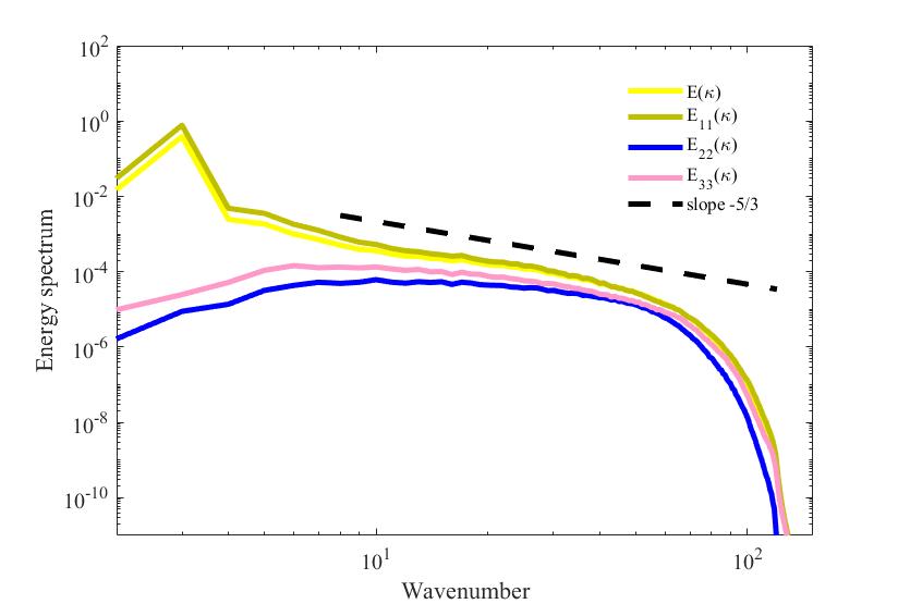
The velocoty spectrum $\Phi_{i j}(\boldsymbol{\kappa})$, as a second-order tensor function, contains a great of information. The simpler form is the energy spectrum $E(\kappa)$. Denote the sphere in wavelength space $\mathcal{S}(\kappa)$, centered at the origon, with radius, $\kappa$. The energy spectrum is defined as,
\[E(\kappa)=\oint \frac{1}{2} \Phi_{i i}(\boldsymbol{\kappa}) \mathrm{d} \mathcal{S}(\kappa)\]Energy spectrum
Alternatively, an equivalent expression through the sifting proper of the Dirac data function is,
\[E(\kappa)=\iint_{-\infty}^{\infty} \frac{1}{2} \Phi_{i i}(\boldsymbol{\kappa}) \delta(|\boldsymbol{\kappa}|-\kappa) \mathrm{d} \boldsymbol{\kappa}\]The velocoty spectrum is from,
\[\Phi_{i j}(\mathbf{\kappa})=F\left\{R_{i j}(\mathbf{r})\right\}\]$F{.}$ is the notation for Fourier transformation. Meanwhile, from the definition of the correlation function,
\[R_{i j}(\mathbf{r})=\left\langle u_{i}(\mathbf{x}) u_{j}(\mathbf{x}+\mathbf{r})\right\rangle\]where $\langle.\rangle$ is the space averging of $\mathbf{x}$.
With Cross-Correlation Theorem, the velocity sprectrum can be expressed as,
\[\Phi_{i j}(\mathbf{\kappa})=F\left\{R_{i j}(\mathbf{r})\right\}=F^{*}\left\{u_{i}(\mathbf{r})\right\} F\left\{u_{j}(\mathbf{r})\right\}=u_{i}^{*}(\mathbf{\kappa}) u_{j}(\mathbf{\kappa})\]The procesures to calculate the enrgy spectrum from the velocity field is,
- Calculate the Fourier transformed field $\mathbf{u}(\mathbf{k})$.
- Calculate $\Phi_{i j}$.
- Calculate the energy spectrum.
Code implementation
The Matlab code for implementation
Suppose the velocity information is stored in three variables, U, V, W as x $\times$ y $\times$ z matrix. The three dimensional Fourier transformation can be conducted as,
amplsU = abs(fftn(U)/numel(U));
amplsV = abs(fftn(V)/numel(V));
amplsW = abs(fftn(W)/numel(W));
The velocity sprectrum with the shifting zero-frequency component to center of spectrum is
EK_U = amplsU.^2;
EK_V = amplsV.^2;
EK_W = amplsW.^2;

EK_U = fftshift(EK_U);
EK_V = fftshift(EK_V);
EK_W = fftshift(EK_W);
The setting of the radius $\mathbf{r}$,
box_radius = int32(ceil((sqrt((box_x)^2+(box_y)^2+(box_z)^2))/2.)+1);

centerx = int32(box_x/2);
centery = int32(box_y/2);
centerz = int32(box_z/2);
Summrize the energy through different radius,
for i = 1:(box_x)
    for j = 1:(box_y)
        for k = 1:(box_z)
            temp = sqrt(double((i-centerx)^2+(j-centery)^2+(k-centerz)^2));
			wn =  int32(round(temp));
            wn = wn+1;
			EK_U_avsphr(wn) = EK_U_avsphr(wn) + EK_U(i, j, k);
			EK_V_avsphr(wn) = EK_V_avsphr(wn) + EK_V(i, j, k);
			EK_W_avsphr(wn) = EK_W_avsphr(wn) + EK_W(i, j, k);
        end
    end
end
The energy sprectrum is,
EK_avsphr = 0.5*(EK_U_avsphr + EK_V_avsphr + EK_W_avsphr);
The figure shows the energy sprectrums.